In this article, we will create a Next-Generation Clustered Heat Map (NG-CHM) of the 200 most variable microRNAs in the TCGA prostate cancer data available from the ISB Cancer Genomics Cloud (ISB-CGC).
We will create the NG-CHM using using our NG-CHM R package, which is available for the RStudio and R software environments. A video introduction to creating NG-CHMs using R is available here. We will use the RStudio environment described in the video.
We will follow these three steps to create the heat map: 1. Download the data from the ISB-CGC. 2. Convert the data into an mirna-by-sample matrix. 3. Create the NG-CHM.
Downloading the Data
To download data from the ISB-CGC you must have a google cloud project with access to the data (see the ISB-CGC documentation for details). Define your project identifier:
myproject <- "Replace with your ISB-CGC project identifier";
We will use the R bigquery package for downloading the ISB-CGC data. ISB-CGC provides some basic documentation for downloading data using R.
To download data using bigquery, you execute an SQL query. Bigquery supports two SQL query formats: standardSQL and legacySQL. We will use standardSQL. StandardSQL is simpler in that it lets you create temporary tables that can then be used to simplify the main query.
We first define a subquery for a temporary table that will contain the SampleBarcodes of the primary tumor prostate cancer samples. TP is the sample type letter code for primary tumor samples. PRAD is the TCGA abbreviation for prostate cancer.
subq1 <- "sample_list AS (
  SELECT SampleBarcode
  FROM `isb-cgc.tcga_201607_beta.Biospecimen_data`
  WHERE SampleTypeLetterCode='TP' AND Study='PRAD' )";
Our second subquery will create a temporary table that includes the miRNA accession identifiers for the 200 miRNAs that vary the most across the samples in the first temporary table.
subq2 <- "miRNA_list AS (
  SELECT mirna_accession, STDDEV(LOG10(normalized_count+1)) AS sigma_log_count
  FROM `isb-cgc.tcga_201607_beta.miRNA_Expression`
  WHERE SampleBarcode IN ( SELECT SampleBarcode FROM sample_list )
  GROUP BY mirna_accession
  ORDER BY sigma_log_count DESC
  LIMIT 200 )"
Our main query uses these two temporary tables to obtain the desired miRNA data:
mainq <- "SELECT SampleBarcode, mirna_id, mirna_accession, LOG10(normalized_count+1) AS log10_count
  FROM `isb-cgc.tcga_201607_beta.miRNA_Expression`
  WHERE
    SampleBarcode IN ( SELECT SampleBarcode FROM sample_list )
    AND mirna_accession IN ( SELECT mirna_accession FROM miRNA_list )"
Assemble and execute the query:
myquery <- paste ("#standardSQL", "WITH", paste (subq1, subq2, sep=", "), mainq, ";", sep="\n");
result <- query_exec (myquery, project=myproject, use_legacy_sql=FALSE);
The returned table includes one row for each matrix element. For example:
result[1:2,]
     SampleBarcode    mirna_id mirna_accession log10_count
1 TCGA-G9-6336-01A hsa-mir-15a    MIMAT0000068    1.606826
2 TCGA-VN-A88O-01A hsa-mir-15a    MIMAT0000068    2.063108
Convert the data into an mirna-by-sample matrix
Recall that in order to create an NG-CHM, the data must be provided as a matrix with row and column labels.
Tidyr’s spread function can map the tuple format returned from bigquery into the required matrix format:
r2 <- tidyr::spread(result, "SampleBarcode", "log10_count");
We extract just the data as a matrix from the spread result:
mirna.raw <- as.matrix(r2[,3:ncol(r2)]);
We must also give the rows of the matrix unique names. Since the mirna_ids are not unique, and the mirna_accession identifiers are not user friendly, we will concatenate the mirna_id and mirna_accession identifiers (separated by a period). This also happens to be the format of the NG-CHM bio.mirna label type.
rownames(mirna.raw) <- sprintf ("%s.%s", r2$mirna_id, r2$mirna_accession);
Create the NG-CHM
As with RNA expression data, differences in base expression levels between miRNAs would dominate the heat map. Therefore, to reduce these differences so that we can focus on relative changes in miRNA levels, we row-center the data:
mirna.rowc <- mirna.raw - apply (mirna.raw, 1, function(x)mean(x));
Finally, we can create and export an NG-CHM containing the data. We also set the row and column axis types, and define the cBioPortal studyid.
hm <- chmNew ('prad-mirna', mirna.rowc, mirna.raw);
hm <- chmAddAxisType (hm, 'row', 'bio.mirna');
hm <- chmAddAxisType (hm, 'column', 'bio.tcga.barcode.sample');
hm <- chmAddProperty (hm, 'cbioportal.study', 'prad_tcga');
chmExportToFile (hm, 'prad-mirna.ngchm', TRUE);
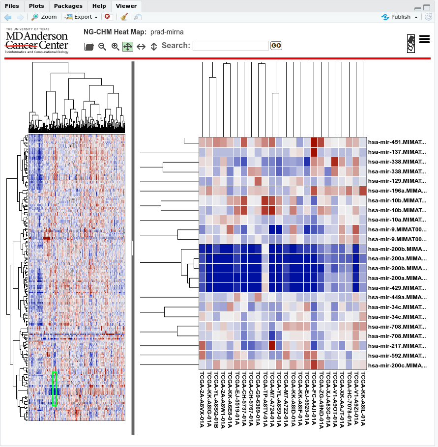
A screenshot of the resulting NG-CHM: